Loading...
Loading...
Loading...
Loading...
Loading...
Loading...
Loading...
Loading...
Loading...
Loading...
Loading...
Loading...
Loading...
Loading...
Loading...
Loading...
Loading...
Loading...
Loading...
Loading...
Loading...
Loading...
Loading...
Loading...
Loading...
Loading...
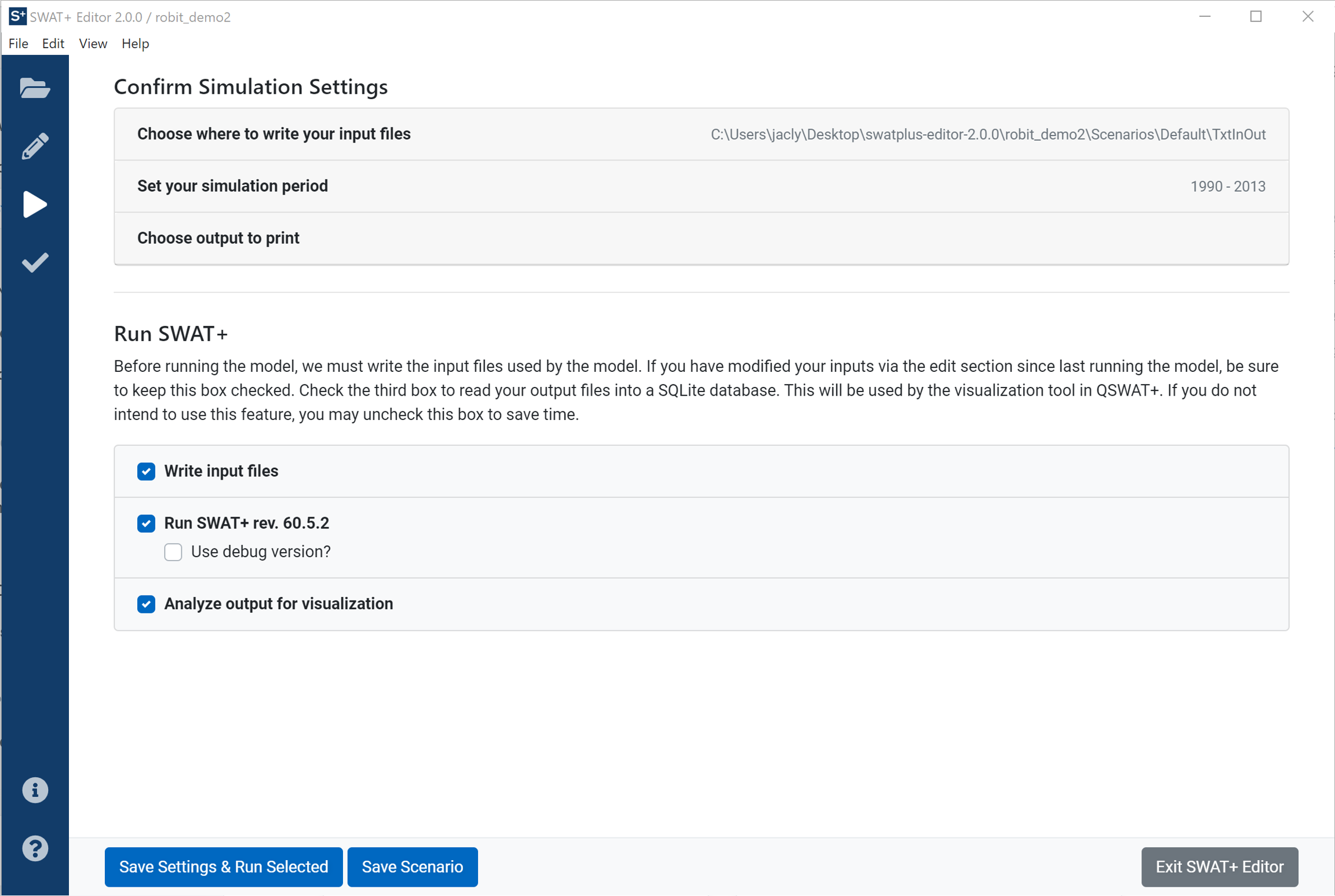
After writing your input files, click the play/triangle button in the leftmost blue toolbar to go to the run SWAT+ section.
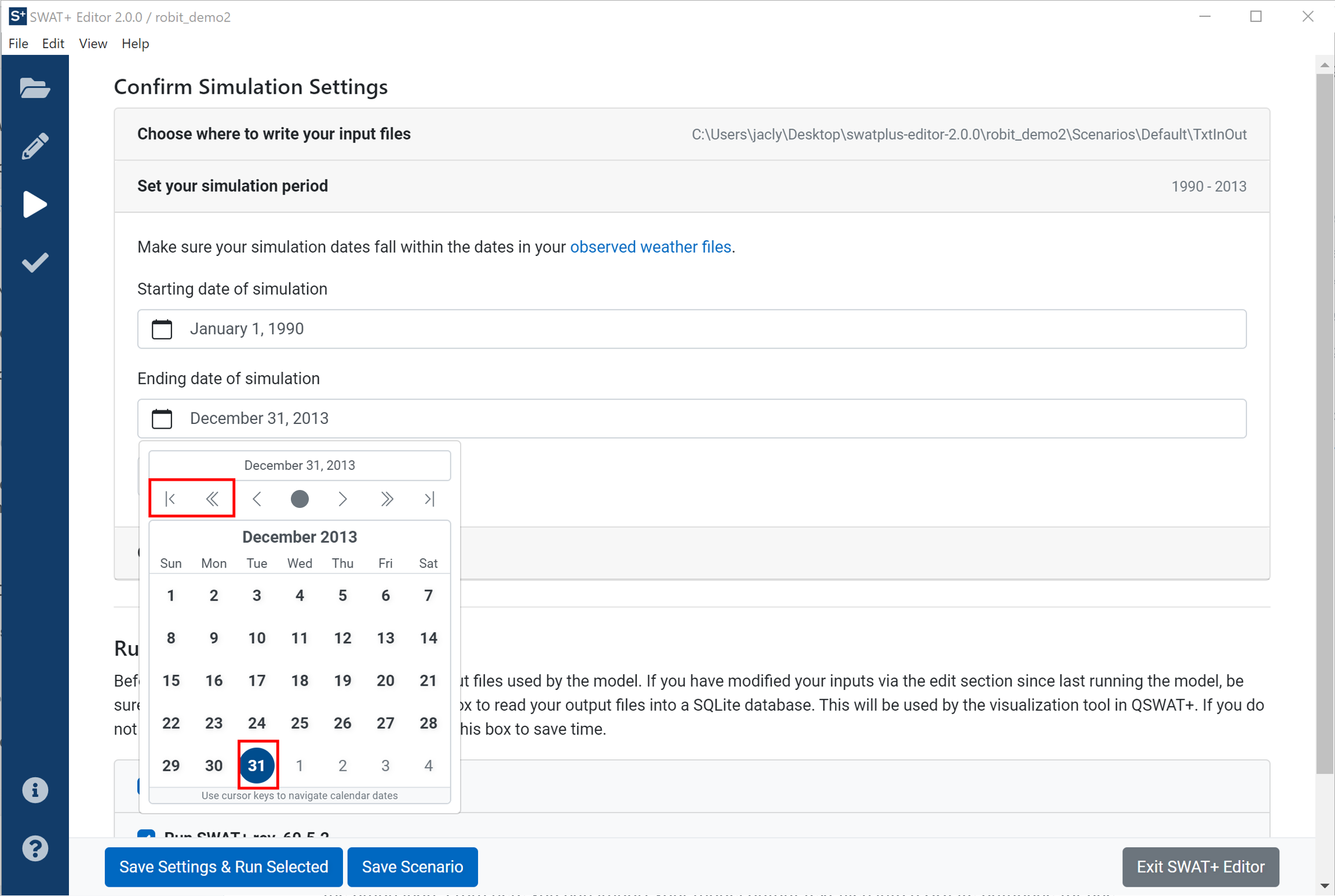
You will see three sections up top to adjust your simulation settings if desired. Your input files will be saved to [Project Directory]/Scenarios/Default/TxtInOut by default. Click on "Set your simulation period" to adjust your starting and ending simulation dates.
When you click on a date picker, please note that you may use the arrows at the top of the date picker to move between decades and years. Then click the day on the calendar to confirm the new date.
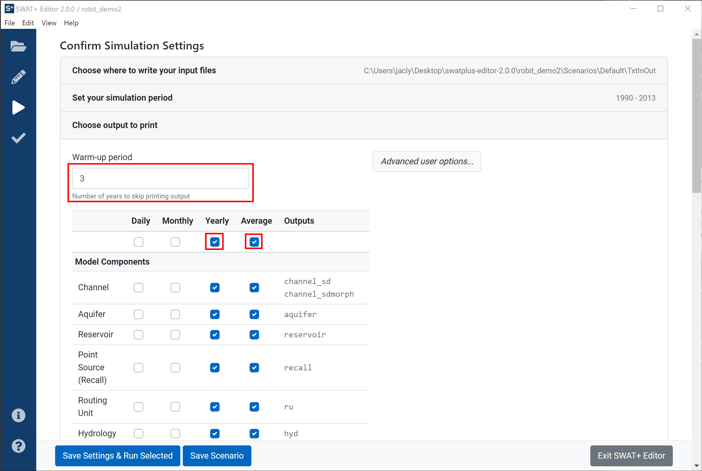
Next you may choose your output to print.
Here is where you set your model warm-up period (2-5 years is recommended) and select which type of output to print. If you intend to use SWAT+ Check, be sure all yearly and annual average files are selected. Use the checkboxes in the top row of the table to select all. Click the advanced user options button on the right for more printing options, such as printing output in CSV. This will print CSV files in addition to the text files that are printed by default.
Collapse the "Choose output to print" section to see the list of run tasks.
Here is a brief description of each task:
Write input files Translate your data saved from the edit inputs section in your project SQLite database to text files read by SWAT+. Any time you make edits, be sure to keep this box checked to re-write your files.
Run SWAT+ Execute a compiled version of the model.
Analyze output for visualization Read the output text files generated by the model into a SQLite database used for SWAT+ check and the QSWAT+ visualization tool
If you encounter an error during the model run, check the box to run the debug version (note: debug is only available on Windows) and run the model again. Copy the contents of the output error and for help diagnosing the problem.
Please refer to the SWAT+ Input/Output Documentation linked below:
Please refer to the SWAT+ Input/Output Documentation linked below:
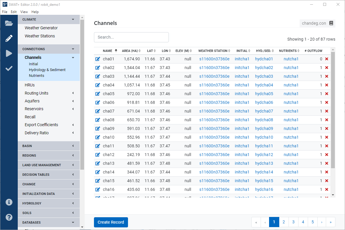
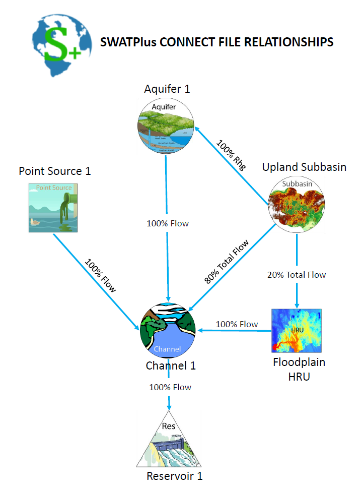
The connections section contains all spatial object connectivity for the simulation run. In SWAT+ Editor, all connection object properties can be set through this section. For example, when you click on channels, you will see additional menu links appear for initialization, hydrology and sediment, and nutrients.
All connection objects have a similar format as seen in the above figure. Each connection object will have properties associated with it (such as initial, hydrology and sediment, and nutrients in this example) as well as a weather station. Click on these names in the table, or from the edit view page, click the button next to their names to view information about the properties object or weather station.
Each connection object may have outflow. The total number of outflow connections is shown in the right-most column of the table (note: you may need to use the horizontal scroll button at the bottom of the table if it is wide). To view the outflow objects, click the edit icon on the left of the row you want to view.
If you imported your project from GIS, your connection objects are populated automatically during project setup.
The subbasin is defined by the DEM in the GIS interface as it always has been. All flow within the subbasin drains to the subbasin outlet.
A landscape unit (LSU) is defined as a collection of HRUs and can be defined as a subbasin, or it could be a flood plain or upland unit, or it could be a grid cell with multiple HRUs. The landscape unit is not routed, it only used for output. The landscape unit output files (waterbal, nutbal, losses, and plant weather) are output for HRUs, landscape units, and for the basin. Two input files are required: 1) landscape elements and, 2) landscape define. The elements file includes HRUs and their corresponding LSU fraction and basin fractions. The define file specifies which HRUs are contained in each LSU.
A routing unit is a collection of hydrographs that can be routed to any spatial object. The routing unit can be configured as a subbasin, then total flow (surface, lateral and tile flow) from the routing unit can be sent to a channel and all recharge from the routing unit sent to an aquifer. This is analogous to the current approach in SWAT. However, SWAT+ gives us much more flexibility in configuring a routing unit. For example, in CEAP, we are routing each HRU (field) through a small channel (gully or grass waterway) before it reaches the main channel. In this case, the routing unit is a collection of flow from the small channels. We also envision simulating multiple representative hillslopes to define a routing unit. Also, we are setting up scenarios that define a routing unit using tile flow from multiple fields and sending that flow to a wetland.
The routing unit is the spatial unit SWAT+ that allows us to lump outputs and route the outputs to any other spatial object. It gives us considerably more flexibility than the old subbasin lumping approach in SWAT, and will continue to be a convenient way of spatial lumping until we can simulate individual fields or cells in each basin.
Documentation for this section is not available yet. For now, please refer to the SWAT+ input/output documentation PDF for parameter definitions.
Weather generator data and weather stations are required for SWAT+ to run.
Weather stations are linked from all of your connection objects (channels, HRUs, etc.) in SWAT+. If you are coming from QSWAT+, it is much better to import stations either from the weather generator section, or the observed weather file importer than it is to create them manually.
By importing through one of the methods described below, your new stations will be automatically matched your spatial connection objects.
Click the import data button to import weather generator (wgn) data for your project. If you installed the SWAT+ databases, this file will be selected by default along with the CFSR world table. USA wgn data is also available from this database; type wgn_us to use this table.
You may also add your own data to this database using the wgn and corresponding wgn_mon tables.
Below the table name field is a check box asking if you are using observed weather data. By default (unchecked), when you click start import, weather stations will be created based on your wgn locations. If you are using observed weather data and prefer to have weather stations created based on this data, check this box--stations will not be created when you start import, and instead they will be created for you when you import your observed weather data files.
If you are not using observed weather data, it is important to leave the box unchecked so that weather stations are created for you.
If you do not want to use the SQLite database, you may import CSV files of your weather generator data. Two CSV files are required.
Stations CSV file:
Columns id, name, lat, lon, elev, rain_yrs
id should be uniquely numbered
Import observed weather data from the top of the weather stations section. The data files may be in one of two formats: SWAT2012/Global Weather Data CFSR website format, or SWAT+.
After importing observed weather data, be sure to check your simulation run time to match your weather dates.
Please ensure the files you're importing are saved with UTF-8 encoding. Otherwise, you may get errors about reading the start date despite it appearing correctly formatted in your files.
You can open your files in Notepad++ and change the encoding via the Encoding menu in the top toolbar. It must be only UTF-8, not other variations.
Each measurement included in your data must have the following entry file names:
Each entry file is a comma-separated list of stations. Each station name should have a corresponding .txt file (e.g., name p326-963 should have a p326-963.txt file).
Each station file should have the first line as the starting day as YYYYMMDD (e.g., 19790101). The following lines are the measurement for each day, one line per day. For temperature, each line will be max,min (e.g., 10.138,-2.662). Please note: SWAT2012 format does not accept hourly data. Please use SWAT+ format described below for hourly weather files.
Global weather data options are available on the .
Each measurement included in your data must have the following entry file names:
Each entry file has a title line (any text allowed), followed by a heading line, followed by a list of filenames for each station. Filenames should be listed alphabetically.
Note: for tmp.cli, we recommend naming your station files with .tem extension instead of .tmp because sometimes Windows will auto-remove files with .tmp extensions thinking they are temporary files. Example:
Each station file has a title line, followed by a heading line and data line for time and location. Measurements for each timestep are in the lines to follow. For temperature, the measurements will be listed as max then min.
For hourly data format, see the .
Each entry in weather_wgn_cli will have 12 rows in weather_wgn_cli_mon.
When entering an observed weather file name in the station editor, you may start typing to search for existing weather files adding during the import step. If adding observed files manually, just type the name of the file (e.g., p326953.pcp), and put that file in the directory you plan to write input files (e.g., your TxtInOut). Files must be in SWAT+ format. If your weather data is in SWAT2012 format or from the Global Weather CFSR website, please use the import step to convert them to SWAT+.
This table is only used if you import observed weather data files. If entering stations manually, this table will not be populated.
Please note: there was a long outstanding issues with time series recall in version 2.0.x of SWAT+ Editor due to a missed change in format of the model. This should be corrected in SWAT+ Editor 2.1.2 and greater. Please update your software and project and reach out if you encounter any issues.
Recall objects are used for connecting point source or inlet data to your watershed. If you added point source in QSWAT+, when you import your project into SWAT+ Editor it will be connected via the recall section.
By default, constant data with all zero values during the default simulation period is added. To add your own recall data, click the recall item in the edit menu under connections.
Please read the README.txt file in the zip carefully.
By default, your recall data is imported as constant. To insert your values, you can edit each item individually by clicking the edit button and manually entering each value. Alternatively, you may upload a CSV of your data.
From the recall section, click the import/export button from the action bar at the bottom. Import is selected by default, so click the export button toggle. Choose a folder name, and click the export data button to get a template for your data.
Constant data will be located in the recall.csv file in the directory you selected. Edit the CSV as needed, save, and then go back to the editor and click the import/output button again. This time toggle the import button. Choose your directory containing your modified files and click the import CSV data button. Your updated values will appear in the table.
By default recall data is imported as constant, however this can be changed by clicking the edit button next to a row in the recall data table. Select the new time step for your data: daily, monthly, or yearly. Click the save changes button. Next, press the back button to go back to the table view. Click the import/export button. Import is selected by default, so click the export button toggle. Choose a folder name, and click the export data button to get a template for your data.
Your directory may now contain two files: a recall.csv containing constant data, and another csv file named for the recall object (e.g., pt002) you changed to time series.
Open the time series file after it is exported to see the template for your data. Modify your data as needed matching the time step you selected previously. Be sure the years match your simulation run time.
You change other recall objects from constant to time series, and you can mix and match all different types (constant, yearly, monthly, and daily). For any recall objects moving from constant to time series, first delete its row in recall.csv. Then create a new csv with the file name matching the recall object's name and insert your time series data. Similarly, if you want to move from time series back to constant, just delete the time series file and add a row back into recall.csv for the object.
To import your data, click the import/export data button again and this time click to toggle import. Choose your directory and click import data. Your new data will appear in the table.
Each record in recall_rec will have a data file named {name}.rec. All of this data is stored in a single recall_dat table in the database.
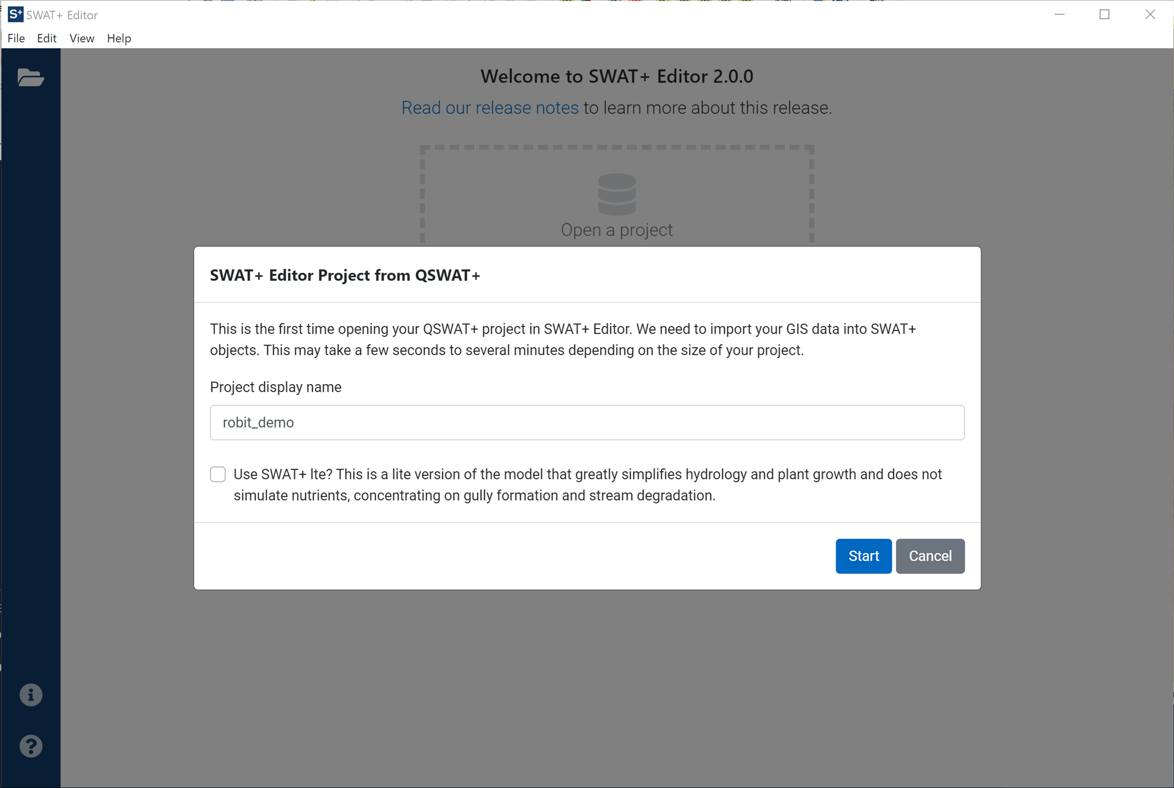
When you open SWAT+ Editor, you are taken to the project setup screen. If you are coming from QSWAT+, an overlay will appear with the option to change your project display name and optionally use the lite version of the mode: SWAT+ lte.
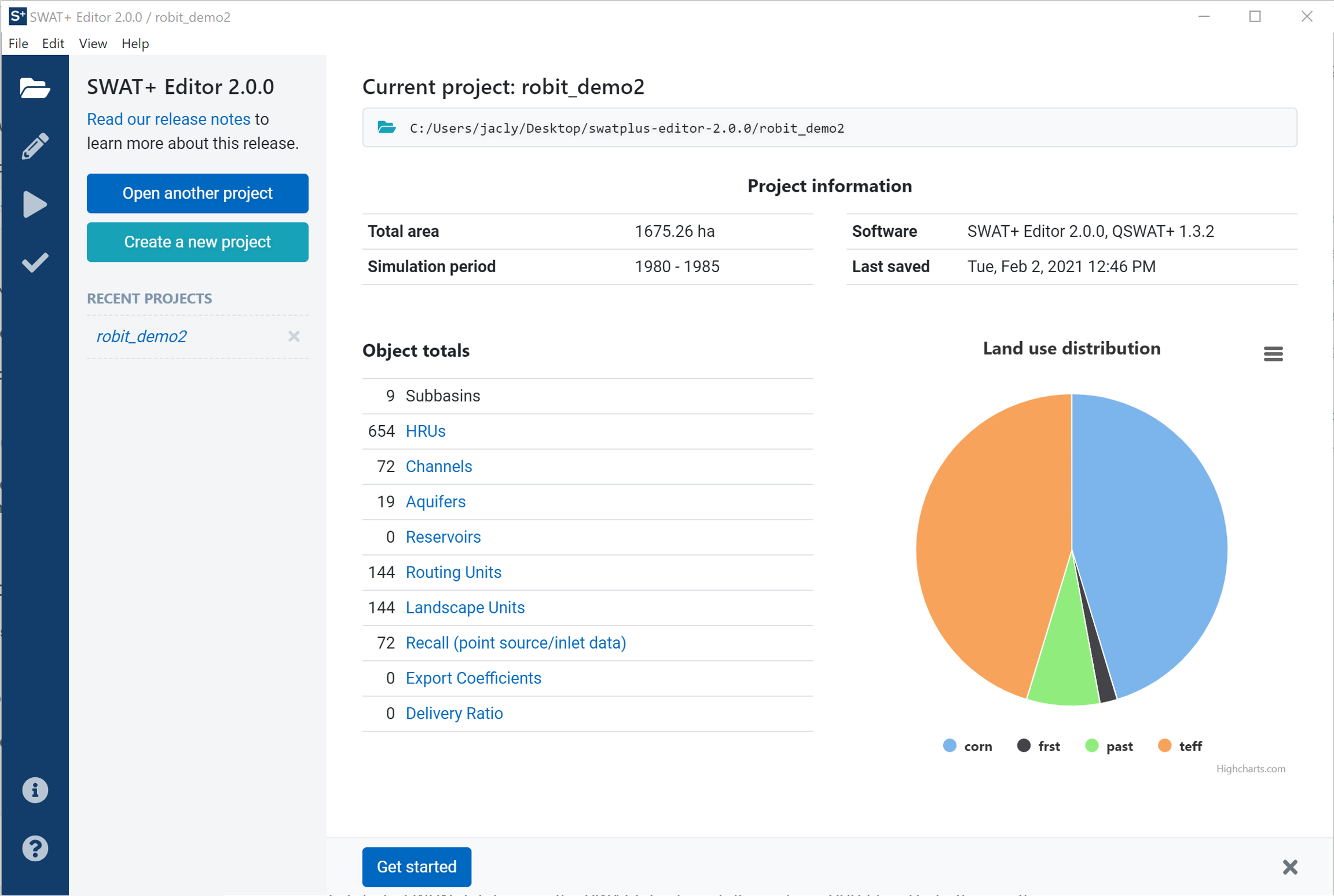
When your project is done importing from GIS, it will be selected as your current project and displayed in the recent projects sidebar on the left as well as in the center screen.
From here you can start editing your SWAT+ inputs by clicking the "Get started" button at the bottom, or by clicking the pencil icon in the far left blue-colored menu.
SWAT+ lte is a version of the SWAT+ model that greatly simplifies hydrology and plant growth and does not simulate nutrients, concentrating on gully formation and stream degradation. It only uses channel and HRU objects.
If you are not coming from QSWAT+, you may open the editor and create a new project from scratch. A project database will be created for you and you will need to input your spatial connections and all other data manually.
Please refer to the SWAT+ Input/Output Documentation linked below:
Please refer to the SWAT+ Input/Output Documentation linked below:
Please refer to the SWAT+ Input/Output Documentation linked below:
Please refer to the SWAT+ Input/Output Documentation linked below:
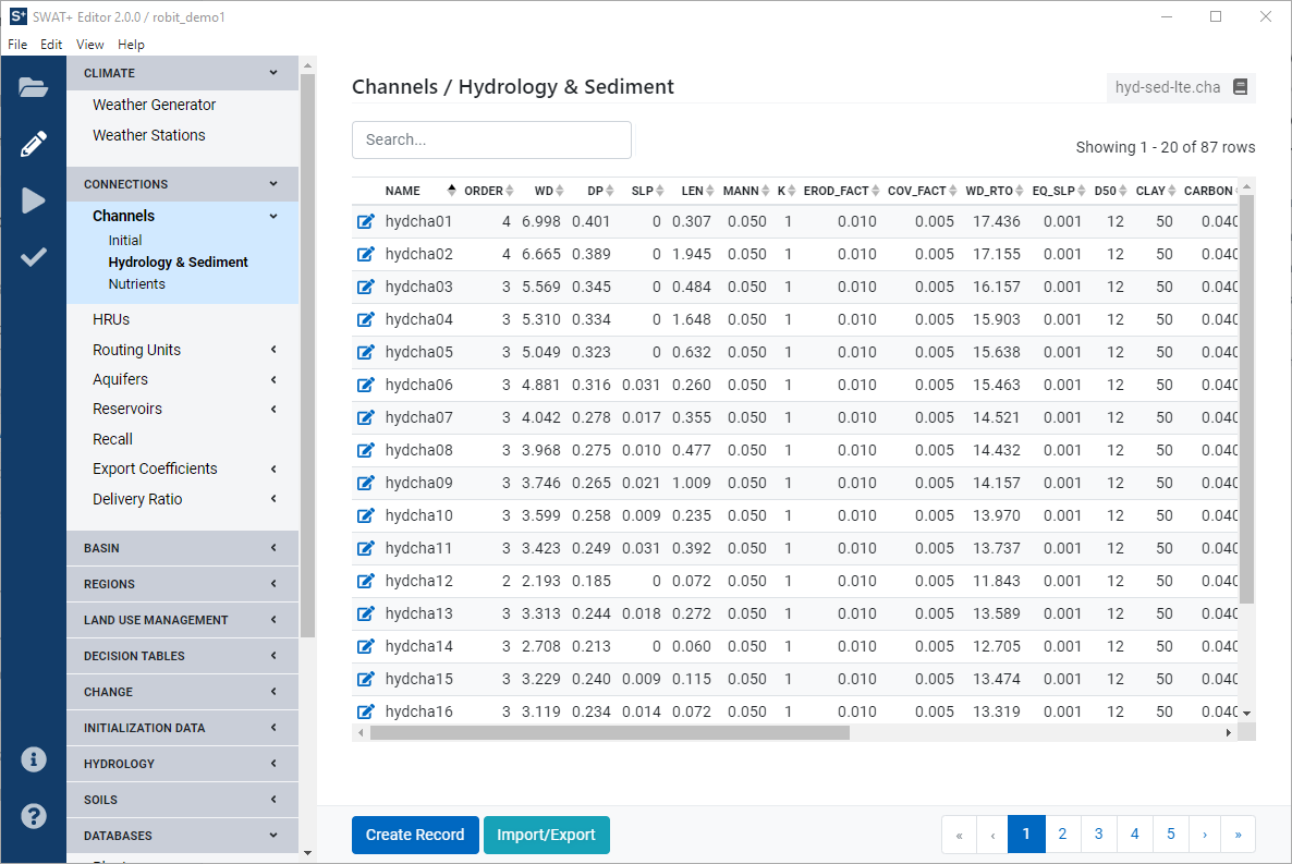
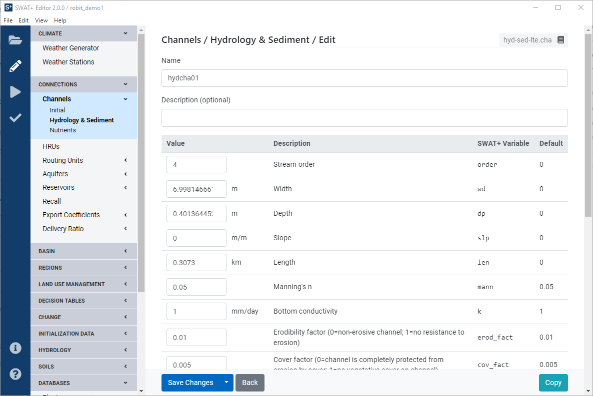
Click the pencil icon in the leftmost blue toolbar to enter the editing section. Most editors in this section are a literal representation of the SWAT+ input files. The collapsible dark-gray headings on the left correspond to the section lines in the master watershed file (file.cio).
When you click on an editor section from the left menu, you'll find the default SWAT+ file name with which the section corresponds. This enables you to quickly look up further information in the SWAT+ input/output documentation.
Most data is presented in a tabular format. When you click a row, you're presented with a form where you can make changes and save. The following features are common across many editor sections.
Sort by a column in the table by clicking on the heading name. It will toggle ascending or descending direction as indicated by the arrows next to the name.
Tables with many records can be scrolled and then paged by clicking the page number or arrow links at the bottom of the table.
Each row may contain an edit/view icon on the far left to access the data in the row, and a delete icon on the far right (may need to scroll to access the far right of the table). We do not recommend deleting rows unless you are absolutely sure they are not used elsewhere in your model. Due to the relationships of data in SWAT+, deleting records could have unintended effects and break your model. Deleting cannot be undone; if in doubt, make a backup of your project SQLite database first.
In the search box up top, start typing the name of the objects you want to find. Matching options will appear in the table. Remove the text from the search box to remove the filter.
In the action bar at the bottom, click create new record to add an item to the table. The import/export data button allows you to quickly access your data in CSV (comma-separated values spreadsheet) format, in most cases. We recommend exporting your data (or empty table is okay) first to get a template with the column names. You may then modify the file and import it back into the editor.
Most objects in SWAT+ have a name field and are identified using this name. Names should be unique and not contain spaces (spaces will be automatically converted to underscores).
Each edit form will have a save changes button at the bottom. Be sure to click this button after making any changes and before leaving the form.
Press the back button to return to the previous screen. Click copy to make a copy of the current object you are viewing. You will be asked to give the copied object a unique name. Note: the copy function is not available for all object types, including connection objects.
There are a lot of relationships between objects in SWAT+. For example, all fields in your channel properties table link to rows in other tables. In SWAT+ Editor forms, you can easily select these related rows by starting to type an object's name and select it as it pops up. If you accidentally enter an incorrect name, the editor will return an error stating the record does not exist in your database.
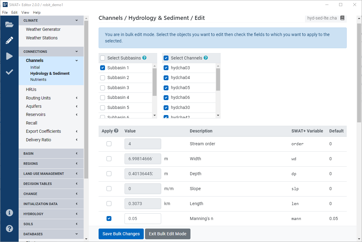
If you want to apply changes to a field for multiple objects at once, you can use bulk edit mode. Select one object from the table as your base. This can be useful if you want to use its values to apply across many other objects, but if you're using entirely new values, it does not matter which object you select.
From the object's edit form page, click the arrow on the right side of the save changes button and then click "Make changes to multiple records..." to enter bulk edit mode.
First, select the objects to which you want to make changes. Note that the object you're currently viewing is not selected by default. For most sections, you can filter your selection by subbasin first. If you're editing an HRU-level objects, you can also filter by landuse. In the above example, we checked Subbasin 1, which then populated the next list with channels that fall into Subbasin 1. All are selected by default, but you can uncheck as needed.
Next, choose which fields you want to edit by clicking the check box to the left of the field. In the above example, we checked the box for Manning's n. Enter the value you want and click Save Bulk Changes. Manning's n will be updated to your new value for each selected channel.
We recommend starting in the climate section, and importing your weather generators and observed weather data. If you're coming from GIS, when you import weather generators or observed data, it will create weather stations and match them to your spatial objects automatically.
A primary goal of environmental modeling is to assess the impact of human activities on a given system. Central to this assessment is the itemization of the land and water management practices taking place within the system. This section contains input data for planting, harvest, irrigation applications, nutrient applications, pesticide applications, and tillage operations. Information regarding tile drains and urban areas is also stored in this file.
Documentation for this section is not available yet. For now, please refer to the SWAT+ input/output documentation PDF for parameter definitions.
In SWAT+, constant values for point sources and inlets are stored in the export coefficients properties file, exco.exc, while time series data are stored entirely in the recall section.
However, in the editor, we keep both constant and time series point sources and inlets in the recall section. When you write input files, the editor will write to the exco.exc and exco_om.exc files appropriately.
Monthly values CSV file:
Columns id, wgn_id, month, tmp_max_ave, tmp_min_ave, tmp_max_sd, tmp_min_sd, pcp_ave, pcp_sd, pcp_skew, wet_dry, wet_wet, pcp_days, pcp_hhr, slr_ave, dew_ave, wnd_ave
id should be uniquely numbered
wgn_id corresponds to the id column from the stations file
lat
real
Latitude of weather station
deg.
+/-90
lon
real
Longitude of weather station
deg.
+/-180
elev
real
Elevation of weather station
m
0-5000
rain_yrs
int
Number of years of recorded maximum monthly 0.5h rainfall data
5-100
month
int
Month
tmp_max_ave
real
Average or mean daily maximum air temperature for month
°C
-30-50
tmp_min_ave
real
Average or mean daily minimum air temperature for month
°C
-40-40
tmp_max_sd
real
Standard deviation for daily maximum air temperature in month
°C
0.1-100
tmp_min_sd
real
Standard deviation for daily minimum air temperature in month
°C
0.1-30
pcp_ave
real
Average or mean total monthly precipitation
mm
0-600
pcp_sd
real
Standard deviation for the average daily precipitation
mm/day
0.1-50
pcp_skew
real
Skew coefficient for the average daily precipitation
mm
-50-20
wet_dry
real
Probability of a wet day after a dry day
0-0.95
wet_wet
real
Probability of a wet day after a wet day
0-0.95
pcp_days
real
Average number of days of precipitation in a month
0-31
pcp_hhr
real
Maximum 0.5 hour rainfall in entire period of record for month
mm
0-125
slr_ave
real
Average daily solar radiation for the month
MJ/m^2/day
0-750
dew_ave
real
Average daily dew point temperature for each month
°C
-50-25
wnd_ave
real
Average wind speed for the month
m/s
0-100
Precipitation gage filename or "sim" if simulated
tmp
text
Temperature gage filename or "sim" if simulated
slr
text
Solar radiation gage filename or "sim" if simulated
hmd
text
Relative humidity gage filename or "sim" if simulated
wnd
text
Wind speed gage filename or "sim" if simulated
wnd_dir
text
Wind direction gage filename
atmo_dep
text
Atmospheric deposition data file name
lat
real
Latitude of weather station
lon
real
Longitude of weather station
Latitude of weather station in file
lon
real
Longitude of weather station in file
Measurement
Entry File
Precipitation
pcp.txt
Temperature
tmp.txt
Solar radiation
solar.txt
Relative humidity
rh.txt
Wind speed
wind.txt
ID
Name
Latitude
Longitude
Elevation
1
p326-963
32.628
-96.250
142.0
Measurement
Entry File
Precipitation
pcp.cli
Temperature
tmp.cli
Solar radiation
slr.cli
Relative humidity
hmd.cli
Wind speed
wnd.cli
pcp.cli: precipitation file names
filename
p326953.pcp
p326956.pcp
tmp.cli: temperature file names
filename
t326953.tem
t326956.tem
SWAT+ Input File
Database Tables
weather-wgn.cli
weather_wgn_cli
weather_wgn_cli_mon
Field
Type
Description
Units
Range
id
int
Auto-assigned identifier
name
text
Name of weather generator
Field
Type
Description
Units
Range
id
int
Auto-assigned identifier
wgn_id
int
ID of row in weather_wgn_cli
SWAT+ Input File
Database Tables
weather-sta.cli
weather_sta_cli
weather_file
Field
Type
Description
id
int
Auto-assigned identifier
name
text
Name of the weather station
wgn_id
int
ID of row in weather_wgn_cli
pcp
Field
Type
Description
id
int
Auto-assigned identifier
filename
text
Name of the weather data file
type
text
Type of weather data: pcp, tmp, slr, hmd, wnd
lat
text
real
yr
int
Year
ob_typ
text
Type of recall
ob_name
text
Name of recall object
flo
real
Volume of water
m^3
sed
real
Sediment
metric ton
orgn
real
Organic nitrogen
kg N
sedp
real
Organic phosphorus
kg P
no3
real
Nitrate
kg N
solp
real
Mineral (soluble P)
kg P
chla
real
Chlorophyll-a
kg
nh3
real
Ammonia
kg N
no2
real
Nitrogen dioxide
kg N
cbod
real
Carbonaceous biological oxygen demand
kg
doc
real
Dissolved oxygen
kg
sand
real
Detached sand
silt
real
Detached silt
clay
real
Detached clay
sag
real
Detached small ag
lag
real
Detached large ag
gravel
real
Gravel
tmp
real
Temperature
deg c
SWAT+ Input File
Database Table
recall.rec
recall_rec
Field
Type
Description
id
int
Auto-assigned identifier
name
text
Name of recall object
rec_typ
int
Time step for recall object (1-daily, 2-monthly, 3-yearly)
SWAT+ Input File
Database Table
{name}.rec
recall_dat
Field
Type
Description
Units
jday
int
Julian day
mo
int
Month
day_mo
int
Day of the month
management_sch_op
cntable.lum
cntable_lum
ovn_table.lum
ovn_table_lum
cons_practice.lum
cons_practice_lum
In addition to the above, SWAT+ Editor groups the operations databases in this section of the editor. However, within the SWAT+ master watershed file (file.cio), these are listed under the ops section.
SWAT+ Input File
Database Table
graze.ops
graze_ops
harv.ops
harv_ops
irr.ops
irr_ops
sweep.ops
sweep_ops
fire.ops
fire_ops
This section is the entry point for management data in SWAT+. It comprises cross-walks to several other sections of data.
This data is accessed from the HRU properties section (hru-data.hru).
Field
Type
Description
Related Table
id
int
Auto-assigned identifier
name
text
Name of the land use properties
cal_group
text
Management schedules comprise auto-schedules (decision tables) and/or operations schedules.
When you import your project from GIS, SWAT+ assigns auto-schedules for management based on your crop land use.
Plant Type (in plants_plt)
Decision Table Template
warm_annual
pl_hv_corn
cold_annual
pl_hv_wwht
perennial
no management schedule
For example, oats is a cold annual crop. If this crop is in your HRUs, a decision table named pl_hv_oats will be created based on the template of pl_hv_wwht when you import your data from GIS.
From the management schedules section, click create a new record or click edit on a row in the table. Give your schedule a unique name.
To add an automatic schedule, start typing a decision table name in the box provided. Click the desired result from the list of matches that pops up, and click the add button. If you enter more than one schedule, you can drag and drop to sort.
To add an operation, click the add operation button. Select your operation type from the form that pops up and complete the remaining fields. Click save when done to add the operation to your table.
When you're done adding automatic schedules and operations, click the save changes button to save your management schedule.
Field
Type
Description
id
int
Auto-assigned identifier
name
text
Name of the schedule
Field
Type
Description
id
int
Auto-assigned identifier
management_sch_id
int
ID of management schedule
d_table_id
int
ID of decision table
Field
Type
Description
id
int
Auto-assigned identifier
management_sch_id
int
ID of management schedule
op_typ
text
Type of operation (see options below)
mon
Code
Description
plnt
plant
harv
harvest only
kill
kill
hvkl
harvest and kill
till
tillage
Code
Value
Look-up Table
plnt
plant name
plants_plt
harv
plant name
plants_plt
kill
plant name
plants_plt
hvkl
Code
Value
Look-up Table
plnt
none
harv
harvest operation name
harv_ops
kill
none
hvkl
Values in the operations tables are provided in the SWAT+ datasets database and copied to your project database during project setup. You may modify them or add new rows as needed in the editor.
SWAT+ Input File
Database Table
harv.ops
harv_ops
Field
Type
Description
Units
id
int
Auto-assigned identifier
name
text
Name of operation
harv_typ
text
SWAT+ Input File
Database Table
graze.ops
graze_ops
Field
Type
Description
Units
Range
id
int
Auto-assigned identifier
name
text
Name of operation
SWAT+ Input File
Database Table
irr.ops
irr_ops
Field
Type
Description
Units
Range
id
int
Auto-assigned identifier
name
text
Name of operation
SWAT+ Input File
Database Table
chem_app.ops
chem_app_ops
Field
Type
Description
Units
id
int
Auto-assigned identifier
name
text
Name of operation
chem_form
text
SWAT+ Input File
Database Table
fire.ops
fire_ops
Field
Type
Description
id
int
Auto-assigned identifier
name
text
Name of operation
chg_cn2
real
Change in SCS curve number II value
frac_burn
SWAT+ Input File
Database Table
sweep.ops
sweep_ops
Field
Type
Description
id
int
Auto-assigned identifier
name
text
Name of operation
swp_eff
real
Removal efficiency of sweeping operation
frac_curb
Values in this table are provided in the SWAT+ datasets database and copied to your project database during project setup. You may modify them or add new rows as needed in the editor.
SWAT+ Input File
Database Table
cntable.lum
cntable_lum
Field
Type
Description
Range
id
int
Auto-assigned identifier
name
text
Name of curve number entry
cn_a
real
Values in this table are provided in the SWAT+ datasets database and copied to your project database during project setup. You may modify them or add new rows as needed in the editor.
SWAT+ Input File
Database Table
cons_practice.lum
cons_practice_lum
Field
Type
Description
id
int
Auto-assigned identifier
name
text
Name of curve number entry
usle_p
real
Usle p factor
slp_len_max
Values in this table are provided in the SWAT+ datasets database and copied to your project database during project setup. You may modify them or add new rows as needed in the editor.
SWAT+ Input File
Database Table
ovn_table.lum
ovn_table_lum
Field
Type
Description
id
int
Auto-assigned identifier
name
text
Name of curve number entry
ovn_mean
real
Overland flow Manning's n = mean
ovn_min
SWAT+ Input File
Database Table
landuse.lum
landuse_lum
management.sch
management_sch
management_sch_auto
Decision tables are a precise yet compact way to model complex rule sets and their corresponding actions. Decision tables, like flowcharts and if-then-else and switch-case statements, associate conditions with actions to perform, but in many cases do so in a more elegant way (see Wikipedia article on decision tables).
Structure of decision tables:
Conditions
Condition alternatives
Actions
Action entries
Each decision corresponds to a variable, relation or predicate whose possible values are listed among the condition alternatives. Each action is a procedure or operation to perform, and the entries specify whether (or in what order) the action is to be performed for the set of condition alternatives the entry corresponds to. Many decision tables include in their condition alternatives the "don’t care" symbol, a hyphen. Using "don’t cares" can simplify decision tables, especially when a given condition has little influence on the actions to be performed. In some cases, entire conditions thought to be important initially are found to be irrelevant when none of the conditions influence which actions are performed.
There are four decision table sections in SWAT+: land use management, reservoir release, scenario land use, and flow conditions.
See the land use management documentation, under management schedules for how to choose a decision table for your HRUs.
Reservoir release decision tables are assigned from the reservoir properties section under connections in SWAT+ Editor.
In the current version of SWAT+ editor, we do not have a GUI available for editing decision tables, however we have provided the ability to export the decision table file. You may then make changes to it in a text editor, and upload back into SWAT+ Editor.
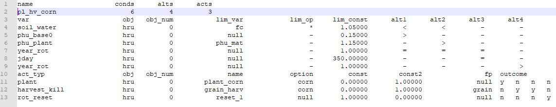
The following is an example of a decision table in the lum.dtl input file. It is a table for warm season annual crops, using continuous corn.
In the above table, there are 6 conditions, 4 alternatives and 3 actions.
soil_water – if soil water is too high (> 1.50*field capacity), it will be too wet to operate machinery
plant_gro – (“n”) Planting allowed if plant is not growing.
phu_base0 – (0.15) when the sum base zero heat units for the year (starting Jan 1) exceeds 0.15, indicating it’s warm enough to plant
If all of the conditions for each alternative are met, outcomes are checked for ‘y’ to take action. Alternatives with dash (‘-‘) are not checked.
plant corn based on heat units: if soil water < 1.50*fc and if phubase0 > 0.15*phu_mat and if year_rot = 1 then check outcomes for ‘y’ and if ‘y’, take that action (plant)
Harvest corn based on crop accumulated heat units: if soil_water < 1.50*fc and if phu_plant > 1.15*phu_mat and if year_rot = 1 and then check outcomes for ‘y’ and if ‘y’, take that action (plant)
Harvest corn based on days since planting: if year_rot = 1 and if days_plant =200 then check outcomes for ‘y’ and if ‘y’, take that action (harvest)
plant: corn – cross walked to plant name in plants.plt file
harvest_kill: corn – cross walked to plant name in plants.plt file grain – relates to harvest type in harv.ops file
rot_reset: rotation reset – for continuous corn (1 year rotation). The rotation year is reset to 1 at the end of every year.
General watershed attributes are defined in the basin input files: codes and parameters. These attributes control a diversity of physical processes at the watershed level. The interfaces will automatically set these parameters to the default or recommended values listed in the variable documentation. Users can use the default values or change them to better reflect what is happening in a given watershed. Variables governing bacteria or pesticide transport need to be initialized only if these processes are being modeled in the watershed. Even if nutrients are not being studied in a watershed, some attention must be paid to these variables because nutrient cycling impacts plant growth which in turn affects the hydrologic cycle.
SWAT+ Input File
Please refer to the SWAT+ Input/Output Documentation linked below:
Please refer to the SWAT+ Input/Output Documentation linked below:
Please refer to the SWAT+ Input/Output Documentation linked below:
Please refer to the SWAT+ Input/Output Documentation linked below:
Please refer to the SWAT+ Input/Output Documentation linked below:
Please refer to the SWAT+ Input/Output Documentation linked below:
Event code
crack
int
Crack flow code
rtu_wq
int
Subbasin water quality code
sed_det
int
Max half-hour rainfall frac calc
rte_cha
int
Water routing method
deg_cha
int
Channel degradation code
wq_cha
int
Stream water quality code
rte_pest
int
Redefined to the sequence number of pest in NPNO(:) to be routed through the watershed
cn
int
CN method flag
c_fact
int
C-factor
carbon
int
Carbon code
baseflo
int
Baseflow distribution factor during the day for subdaily runs
uhyd
int
Unit hydrograph method
sed_cha
int
Instream sediment model
tiledrain
int
Tile drainage EQ code
wtable
int
Water table depth algorithms code
soil_p
int
Soil phosphorus model
abstr_init
int
Initial abstraction on impervious cover
atmo_dep
text
Atmospheric deposition code
stor_max
int
Max depressional storage selection code
headwater
int
Headwater code
0
0-1
surq_lag
real
Surface runoff lag coefficient
4
1-24
adj_pkrt
real
Peak rate adjustment factor for sediment routing in the subbasin (tributary channels)
1
0.5-2
adj_pkrt_sed
real
Peak rate adjustment factor for sediment routing in the main channel
1
0-2
lin_sed
real
Linear parameter for calculating the maximum amount of sediment that can be reentrained during channel sediment routing
0.0001
0.0001-0.01
exp_sed
real
Exponent parameter for calculating sediment reentrained in channel sediment routing
1
1-1.5
orgn_min
real
Rate factor for humus mineralization of active organic nutrients (N and P)
0.0003
0.001-0.003
n_uptake
real
Nitrogen uptake distribution parameter
20
0-100
p_uptake
real
Phosphorus uptake distribution parameter
20
0-100
n_perc
real
Nitrate percolation coefficient
0.2
0-1
p_perc
real
Phosphorus percolation coefficient
10 m^3/M
10
10-17.5
p_soil
real
Phosphorus soil partitioning coefficient
m^3/Mg
175
100-200
p_avail
real
Phosphorus availability index
0.4
0.01-0.7
rsd_decomp
real
Residue decomposition coefficient
0.05
0.02-0.1
pest_perc
real
Pesticide percolation coefficient
0.5
0-1
msk_co1
real
Calibration coefficient to control impact of the storage time constant for the reach at bankfull depth
0.75
0-10
msk_co2
real
Calibration coefficient used to control impact of the storage time constant for low flow (where low flow is when river is at 0.1 bankfull depth) upon the km value calculated for the reach
0.25
0-10
msk_x
real
Weighting factor control relative importance of inflow rate and outflow rate in determining storage on reach
0.2
0-0.3
trans_loss
real
Fraction of transmission losses from main channel that enter deep aquifer
0
0-1
evap_adj
real
Reach evaporation adjustment factor
0.6
0.5-1
cn_co
real
Currently not being used
denit_exp
real
Denitrification exponential rate coefficient
1.4
0-3
denit_frac
real
Denitrification threshold water content
1.3
0-1
man_bact
real
Fraction of manure applied to land areas that has active colony forming units
0.15
0-1
adj_uhyd
real
Adjustment factor for subdaily unit hydrograph basetime
0
0-1
cn_froz
real
Parameter for frozen soil adjustment on infiltration/runoff
0.000862
0-0
dorm_hr
real
Time threshold used to define dormancy
hrs
0
0-24
s_max
real
Currently not being used
n_fix
real
Nitrogen fixation coefficient
0.5
0-1
n_fix_max
real
Maximum daily-n fixation
kg/ha
20
1-20
rsd_decay
real
Minimum daily residue decay
0.01
0-0.05
rsd_cover
real
Residue cover factor for computing fraction of cover
0.3
0.1-0.5
vel_crit
real
Critical velocity
5
0-10
res_sed
real
Reservoir sediment settling coefficient
0.184
0.09-0.27
uhyd_alpha
real
Alpha coefficient for gamma function unit hydrograph
5
0.5-10
splash
real
Splash erosion coefficient
1
0.9-3.1
rill
real
Rill erosion coefficient
0.7
0.5-2
surq_exp
real
Exponential coefficient for overland flow
1.2
1-3
cov_mgt
real
Scaling parameter for cover and management factor for overland flow erosion
0.03
0.001-0.45
cha_d50
real
Median particle diameter of main channel
mm
50
10-100
cha_part_sd
real
Geometric standard deviation of particle size
1.57
1-5
adj_cn
real
Currently not being used
igen
int
Random generator code 0 = use default number; 1 = generate new numbers in every simulation
0
0-1
Database Table
codes.bsn
codes_bsn
Field
Type
Description
pet_file
text
Potential ET filename
wq_file
text
Watershed stream water quality filename
pet
int
Potential ET method code
event
SWAT+ Input File
Database Table
parameters.bsn
parameters_bsn
Field
Type
Description
Units
Default
Range
lai_noevap
real
Leaf area index at which no evaporation occurs from water surface
3
0-10
sw_init
real
int
Initial soil water storage expressed as a fraction of field capacity water content
obj
text
Object variable (res, hru, etc)
obj_num
int
Object number
lim_var
text
Limit variable (evol, pvol, fc, etc)
lim_op
text
Limit operator (*, +, -)
lim_const
real
Limit constant
obj
text
Object variable (res, hru, etc)
obj_num
int
Object number
name
text
Name of action
option
text
Action option-specific to type of action (e.g., for reservoir, option to input rate, days of draw-down, weir equation pointer, etc)
const
real
Constant used for rate, days, etc
const2
real
fp
text
Pointer for option (e.g., weir equation pointer)
year_rot – needed to identify the current year of rotation. In this example, corn is grown in year 1.
days_plant – days since last plant (200) to ensure harvest occurs before next crop is planted.
SWAT+ Input File
Database Table
lum.dtl, res_rel.dtl, scen_lu.dtl, flo_con.dtl
d_table_dtl
d_table_dtl_cond
d_table_dtl_cond_alt
d_table_dtl_act
d_table_dtl_act_out
Field
Type
Description
id
int
Auto-assigned identifier
name
text
Name of the decision table
file_name
text
File name denoting type of decision table: lum.dtl, res_rel.dtl, scen_lu.dtl, flo_con.dtl
Field
Type
Description
Related Table
id
int
Auto-assigned identifier
d_table_id
int
ID of decision table
d_table_dtl
var
text
Field
Type
Description
Related Table
id
int
Auto-assigned identifier
cond_id
int
ID of condition
d_table_dtl_cond
alt
text
Field
Type
Description
Related Table
id
int
Auto-assigned identifier
d_table_id
int
ID of decision table
d_table_dtl
act_typ
text
Field
Type
Description
Related Table
id
int
Auto-assigned identifier
act_id
int
ID of action
d_table_dtl_act
outcome
bool
Condition variable
Condition alternatives (>, <, =)
Type of action (reservoir, irrigate, etc)
Perform action (1 or true), or don't perform action (0 or false)
chem_app.ops
chem_app_ops
Calibration group
plnt_com_id
int
Plant community
plant_ini
mgt_id
int
Management schedule
management_sch
cn2_id
int
Curve number
cntable_lum
cons_prac_id
int
Conservation practices
cons_prac_lum
urban_id
int
Urban land use
urban_urb
urb_ro
text
Urban runoff
ov_mann_id
int
Overland flow Manning's n
ovn_table_lum
tile_id
int
Tile drain
tiledrain_str
sep_id
int
Septic tank
septic_str
vfs_id
int
Filter strip
filterstrip_str
grww_id
int
Grassed waterway
grassedww_str
bmp_id
int
Best management practices
bmpuser_str
description
text
Optional description of the row
int
Month operation takes place
day
int
Day operation takes place
op_data1
text
Dependent on op_typ (see options below)
op_data2
text
op_data3
real
Override value
irrm
irrigation
fert
fertilizer
pest
pesticide application
graz
grazing
burn
burn
swep
street sweep
prtp
print plant vars
skip
skip to end of the year
plant name
plants_plt
till
tillage name
tillage_til
irrm
irrigation operation name
irr_ops
fert
fertilizer name
fertilizer_frt
pest
pesticide name
pesticide_pst
graz
graze operation name
graze_ops
burn
fire operation name
fire_ops
swep
street sweep operation name
sweep_ops
prtp
none
skip
none
harvest operation name
harv_ops
till
none
irrm
none
fert
chemical application operation name
chem_app_ops
pest
chemical application operation name
chem_app_ops
graz
none
burn
none
swep
none
prtp
none
skip
none
Harvest type: grain, biomass, residue, tree, or tuber
harv_idx
real
Harvest index target specified at harvest
harv_eff
real
Harvest efficiency
harv_bm_min
real
Minimum biomass to allow harvest
kg/ha
description
text
Optional description
fert_id
int
ID of fertilizer from fertilizer_frt
bm_eat
real
Dry weight of biomass removed by grazing daily
kg/ha
0-500
bm_tramp
real
Dry weight of biomass removed by trampling daily
kg/ha
0-500
man_amt
real
Dry weight of manure deposited
kg/ha
0-500
grz_bm_min
real
Minimum plant biomass for grazing to occur
kg/ha
0-5000
description
text
Optional description
irr_eff
real
Irrigation efficiency
0-1
surq_rto
real
Surface runoff ratio
0-1
irr_amt
real
Depth of application for subsurface
mm
0-100
irr_salt
real
Concentration of salt in irrigation water
mg/l
irr_no3n
real
Concentration of nitrate in irrigation water
mg/l
irr_po4n
real
Concentration of phosphate in irrigation water
mg/l
description
text
Optional description
Chemical form: liquid or solid
app_typ
text
Application type: spread, spray, inject, direct
app_eff
real
Application efficiency
foliar_eff
real
Foliar efficiency
inject_dp
real
Injection depth
mm
surf_frac
real
Surface fraction amount in upper 10mm
drift_pot
real
Drift potential
aerial_unif
real
Aerial uniformity
description
text
Optional description
real
Fraction burned
description
text
Optional description
real
Fraction of the curb length that is sweep-able
description
text
Optional description
Curve number for hydrologic soil group A
30-100
cn_b
real
Curve number for hydrologic soil group B
30-100
cn_c
real
Curve number for hydrologic soil group C
30-100
cn_d
real
Curve number for hydrologic soil group D
30-100
description
text
Optional description
treat
text
Treatment/Practice
cond_cov
text
Condition of cover
real
Maximum slope length
description
text
Optional description
real
Overland flow Manning's n = min
ovn_max
real
Overland flow Manning's n = max
description
text
Optional description
Download example data formatted for importing into the editor
Some files below may be zipped. Please unzip before using in the editor.
Climate
Weather Generator
Formats not included in this page can usually be found by using the import/export tool on each table in SWAT+ Editor. Export the current data to CSV to get the template.

Climate
Weather Stations
Climate
Atmospheric Deposition
Connections
Point Source / Inlet


Water allocation tables are very specific to the watershed and new feature in SWAT+. We recommend working with the model development team if you are unsure. Because this is a new addition, the interface is still limited if you're trying to build a large table with many source and demand objects.
Field
Description
Type
name
name of the water allocation object
string
rule_typ
rule type to allocate water
Demand. Demand can be irrigation demand from an hru, municipal demand, or demand to transfer to another source object (channel, reservoir, aquifer). For irrigation demand, the hru number, decision table for triggering irrigation, and irrigation depth (mm) are input. For municipal demand, a muni number is input. The user then has the option to input an average daily demand or a recall name that can be daily, monthly, or annual. For transfer demand, the trans number is input and the user can input an average daily demand or a decision table to specify demand.
Treatment. Treatment is designed for municipal treatment plants or industrial plants that treat or change the water chemistry. There are 2 options – 1) recall where you can specify the amount of return flow and 2) delivery where you can specify the change in flow and chemistry.
Receiving. This can be used to return the treated municipal water (point sources) or to transfer (divert) water to other objects. The simple option is the input the return object and number. Or a decision table can be input to condition the diversions to multiple objects. Inputting “lost” assumes the water is diverted out of the basin.
Source Allocation. The sources are listed in order of selection and the fraction from each source is input. The other input is compensation – if other sources are not available, the current source may be allowed to compensate for the demand. The model goes through all sources in the order listed and allocates based on the fractions. The model loops through the sources again, checking to see if compensation is allowed
real
string
amount
m3 per day for muni and mm for HRU
real
right
water right (sr=senior; jr=junior)
string
treat_typ
recall for inputting a recall object and treat for a treatment object
string
treatment
pointer to the recall or delivery ratio file
string
rcv_ob
receiving object (channel, reservoir, aquifer) - no decision table, all return to this object
string
rcv_num
receiving object number
integer
rcv_dtl
receiving object decision table - to condition water transfers and diversions
string
dmd_src_obs
number of source objects available for the demand object
integer
string
src_obs
number of source objects
integer
dmd_obs
number of demand objects
integer
cha_ob
channel object (enter y=yes there is a channel object; enter n=no channel object (only one per water allocation object)
string
Field
Description
Type
num
demand object number
integer
ob_typ
object type (channel=cha; reservoir=res; aquifer=aqu; unlimited source=unl)
string
ob_num
number of the object type
integer
limit_mon
Field
Description
Type
num
demand object number
integer
ob_typ
hru (for irrigation) or muni (muncipal) or divert (interbasin diversion)
string
ob_num
number of the object type
integer
withdr
minimum monthly values for object type:
channel flow (m3/s)
minimum reservoir level (fraction principal);
maximum aquifer depth (m);
withdrawal type - average day or recall for muni and divert; irrigation for HRU